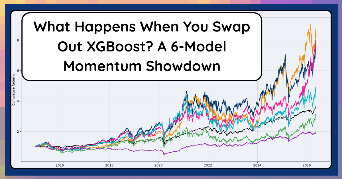
What Happens When You Swap Out XGBoost? A 6‑Model Momentum Showdown

Disclaimer: Quant Science is not a registered investment adviser under the Investment Advisers Act or a commodity trading advisor under the Commodity Exchange Act. The information provided is for educational and informational purposes only and does not constitute investment, financial, or trading advice.

Disclosure: This post contains affiliate links. I am an affiliate for Quant Science and may receive a commission if you sign up or make a purchase using my links. I’d appreciate it if you used them—there’s no additional cost to you, and in some cases it may even give you a discount. All opinions are my own and based on my personal experience with the course and tools.

Every time I post about my XGBoost‑based momentum strategy, someone asks, “Why not LightGBM?” or “Why not CatBoost?” After 16 years of building ML systems, that sounds like a good time. I swapped the algorithms to see what actually changes in my trading system. Changing out the models in this setup is simple. Here we’ll look at how a few major algorithm families behave in the same momentum system: gradient boosted trees (GBMs), a bagged tree (random forest), a linear model, and a simple neural net.

My goals for this experiment were straightforward: keep the data, features, filters, and backtest setup identical; swap only the model and use reasonable defaults; and log everything to MLflow so I can compare runs cleanly and share screenshots and metrics. 

Here's where we're going :

• The models we’re comparing

• My hypothesis and some history

• Methodology, backtest & data assumptions

• Results

• How did I swap out the models (code)

• Conclusion

Algorithms I Compared

Here’s the lineup:

• XGBoost – Original baseline GBM this system was built around; strong performance and my default choice up to now.

• LightGBM – Drop‑in gradient boosting replacement, optimized for speed and large tabular datasets.

• CatBoost – Gradient boosting with native categorical handling and symmetric (oblivious) trees.

• Random Forest – Classic bagged decision trees, no boosting; a natural pre‑GBM workhorse and sanity‑check ensemble.

• LASSO – Linear model with L1 regularization on scaled inputs; interpretable, sparse baseline.

• Neural Net (MLPRegressor) – Simple feedforward network on scaled inputs; a non‑tree, non‑linear benchmark to see how a basic NN behaves in this setup.

My hypothesis and some history

My hypothesis:

I expected the GBMs to perform similarly and to outperform the LASSO and random forest models. If you’d forced me to rank them beforehand, I’d have put LASSO at the bottom, random forest and the neural net somewhere in the middle (I wasn’t quite sure how a two‑layer NN would perform), and the GBMs at the top.

High‑Level, Why This Was My Hypothesis (feel free to skip if you just want results) :

If you were modeling before XGBoost showed up around 2014, you were probably in love with random forests. They were the Swiss Army knife of tabular ML: fewer assumptions than logistic regression, solid performance out of the box, and relatively little tuning. A lot of us were also shifting from plain logistic regression to LASSO. LASSO kept the linear structure but added a penalty that shrinks unimportant coefficients toward zero, which solved some of the overfitting and p‑hacking problems that came with stepwise regression. By the early 2010s, LASSO became a go‑to when you needed something interpretable but also needed to reduce your feature set.

At the same time, neural nets were powerful but still felt like overkill for many tabular problems. They were often considered over‑engineering for common modeling use cases: they were seen as a black box, required more compute, and in many organizations, more interpretable models were preferred. I was building neural nets in 2010 in the utilities, but my later roles shied away from them for exactly these reasons. If you needed to ship something explainable, you would reach for logistic regression, LASSO, or a single decision tree like CART or CHAID.

Then gradient boosting hit the scene. As GBMs like XGBoost arrived, they started to dominate any problem where pure predictive accuracy mattered, because they could capture nonlinear interactions and complex effects that linear models and bagged trees missed—without demanding neural‑net levels of compute or infrastructure. In a lot of tabular settings, GBMs became the practical middle ground: more flexible than linear models, but easier to train, deploy, and justify than a neural net. You still reached for LASSO when you truly needed to understand the marginal effect of each feature and explain it to non‑technical stakeholders, because modern explainability tools were not yet accessible.

As feature importance, partial dependence, and SHAP became standard, that trade‑off softened: you could get GBM‑level performance and still say something concrete about which features mattered and in what direction. LightGBM (from Microsoft) and CatBoost (from Yandex), both released around 2017, refined gradient boosting with faster training, better handling of sparse and categorical inputs, and their own innovations in tree structure. For most tabular prediction problems today, you just reach for your favorite GBM, and as long as your data and pipeline are solid, that choice rarely makes or breaks performance.

Methodology, backtest, and data assumptions 

Most of the features and filters I’m using here come from the concepts taught in the Quant Science course. 

Data & timeframe

• Started January 1, 2015. My production backtests go back to 2000, but 11 years felt sufficient for comparison in this example.

• NYSE daily data.

• A recent 2‑year lookback window for screening (signals are fit and then evaluated forward from there).

• If you rerun this over the same period with a different random seed, you should expect some variability in the metrics.

Universe & filters

• Liquidity and volatility constraints (volume, price, and risk filters).

• Basic quality / growth style filters (for example, “Rule‑of‑40”‑type metrics, cash‑flow and growth screens).

Feature set

• Technical trend and momentum indicators (MACD‑style signals, momentum, ROC, RSI, regime markers).

• Fundamental metrics covering growth, profitability, leverage, and cash flow.

• Additional interaction and regime factors.

Portfolio construction

• Long‑only, rules‑based selection of top candidates with weighted positions.

• Transaction costs and slippage explicitly modeled.

Model‑specific assumptions and caveats

• This entire pipeline was originally built and iterated on using XGBoost. The features, filters, and universe selection were all developed while evaluating and optimizing XGBoost performance. In other words, XGBoost has a home‑field advantage in this comparison, and you should read its performance with that bias in mind. 

• Random forest is run with n_jobs = -1, which tells it to use all available cores; the GBMs already default to multi‑threaded training, but without parallelism, random forest would have taken even longer (than 4.7 hours) to run.

• All GBMs use near‑default settings. I removed any custom parameters I had previously set for XGBoost so the GBMs are all comparable. 

• The neural net uses two hidden layers (64 and 32 neurons) with an otherwise simple configuration.

• LASSO and the neural net both need clean, scaled numeric inputs, so I applied imputation and scaling before training them.

Results:

This chart shows cumulative returns for all six algorithms from January 2015 through May 2026. The only thing that changed between runs was the model. The S&P 500 is included as a reference. All of the GBMs and the neural net beat the S&P (even with just the defaults), while LASSO and random forest did not. Now we’ll dig a little deeper into how and where those differences show up, and a few places they surprised me.… 

All runs share the same benchmark metrics, confirming the setup was identical across models. Below is the same information, but easier to read.

XGBoost and LightGBM tell a similar story on CAGR and total return, but XGBoost pulls ahead on risk‑adjusted metrics: its Sharpe is meaningfully higher, and its max drawdown is shallower. The neural net actually edges out both on CAGR, total return, and Sortino, but it pays for that with a significantly deeper max drawdown. CatBoost is the most disappointing of the GBM family here, with the lowest total return and the worst max drawdown among the boosted trees. Random forest and LASSO lag all of the GBMs and the neural net on CAGR, Sortino, total return, and Sharpe. 

However, when we look at average drawdown by average up month (chart below), CatBoost holds its own. It lags the other GBMs with lower total return and a deeper max drawdown, but its average month‑to‑month returns look similar. 

The neural net is actually the standout in several ways: highest CAGR (0.202), highest Sortino (1.458), and highest total return (7.089) of all six models. That said, its Sharpe (0.628) and YTD (0.065) tell a more complicated story: strong performance over the full backtest period, but weak performance in the current market regime. The YTD gap tells that story clearly: 0.065 vs XGBoost’s 0.458.​​​​​​​​​​​​​​​​

Random forest tells a straightforward story: it didn’t beat the S&P over the full backtest period, and its risk-adjusted metrics are the weakest of the non-linear models. A CAGR of 0.099, Sharpe of 0.522, and Sortino of 0.849 all trail the GBMs by a meaningful margin. I set n_jobs=-1 to speed things up, and it still took 4.7 hours. That’s more than twice as long as the next longest model, the Neural Net.​​​​​​​​​​​​​​​​

LASSO performed the worst and underperformed the S&P. But I’m not surprised that a linear model would have difficulty capturing momentum dynamics.

The GBMs deliver the most attractive mix of return and risk, and the neural net may be a volatile overachiever based on its YTD relative to its full-period metrics. The simpler models mostly confirm what we'd expect. Now let's dig into how I ran these comparisons, and why swapping models in this system isn't difficult. 

---

Attend the Next Quant Science Webinar

In this webinar, you’ll hear all about what it takes to manage and start working with an end-to-end algo trading pipeline.

What: Algorithmic Trading for Data Scientists

How It Will Help You: Learn how the Quant Science course would teach you how to build, backtest, and track systematic trading strategies using tools like Python, Zipline, and MLflow, so you can confidently experiment, refine, and grow as a trader.

Price: Free

How To Join:  Register Here

---

How Easy It Was to Swap Models

To give one concrete example, here’s what it took to switch from XGBoost to LightGBM:

1. pip install lightgbm

2. In my algorithms module, I added a function like:

Then you’ll import your helper function from the algorithms script. You’ll also need to define the model parameters in your config:

There were only a couple of other places where I updated naming conventions, and that was it. This snippet also leaves out how I logged the model and metadata to MLflow, but I wanted to keep the focus on what is involved in switching out the model. If you haven’t used MLflow yet and you’re doing any kind of backtesting or experiment tracking, it’s like the free, detailed journal you already know you need in your life. I’ve written about the benefits of MLflow here.

Swapping all of the other models followed basically the same pattern, with the small exception that LASSO and the neural net needed some imputation and scaling (but that wasn’t much code either). If you take anything away from this section, let it be this: for well‑designed systems, the model is a small, swappable component.

Conclusion:

Going in, I expected the GBMs to be pretty interchangeable, with LASSO at the bottom. That broad picture held up, but CatBoost was weaker than I expected, and the neural net had this odd “great long‑term, terrible recent” profile that can look good in a table but isn’t something I’d trust in the current regime.

The next steps would be pretty standard: take the top couple of candidates (for me, XGBoost and LightGBM), do some manual, risk-aware hyperparameter exploration, and validate them in walk‑forward backtests and analysis. The goal here was to understand how different algorithms behave when you plug reasonable defaults into the same pipeline, not to squeeze every last basis point out of a single model. I’m also happy to continue working with XGBoost for my system.

For someone who’s new to ML in trading, I hope this is encouraging. You can grab a reasonable algorithm and start. If your data pipeline, features, and risk controls are solid, most modern GBMs will already get you into a pretty good ballpark, and you can always change or tune the model later.

If you want to go deeper into the framework behind this system—universe filters, feature engineering, and risk controls—those ideas come from the Quant Science course I mentioned earlier. You can check it out here; that’s an affiliate link, which helps support my writing at no extra cost to you.